Theory

The segmentation path graph

To simplify the logic of handling intervals, it is common practice in sequence analysis to use a 0-based coordinate system that labels individual nucleotides, or ranges of nucleotides, by the coordinates that flank them. Similarly, we define here a 0-based coordinate system for genomic bins that labels individual bins by their edges (Fig. 3).

Fig. 3

Top: Coordinate systems for a binned genomic region: segmentations are unambiguously expressed in a 0-based or “edge-based” representation that designates which bin edges are the boundaries between segments of genomic bins. Bottom: example segmentation (red lines) expressed in binary notation.

For a symmetric genomic interaction heatmap (the same coordinates on both axes), we have an ordered list of contiguous genomic bins, each of which is an interval of one or more bases, represented by the following bin edge labels:

\[V = (0,1,2,\ldots, N).\]

We define a segment as a set of consecutive bins according to the sequence \(V\).

We define a segmentation \(s\) as a collection of non-overlapping segments that covers \(V\) (i.e., no repeated bins, no gaps).

We denote \(S\) the state space of all segmentations over \(V\).

In this coordinate system, any segment can be represented as a half-open interval, denoted by pairs \([a,b)\), where \(a \lt b\). For example, the first bin is denoted \([0,1)\), the segment spanning the first five bins is denoted \([0,5)\). We can represent segmentations in several ways:

1. as sets of adjacent half-open intervals (e.g., \(\\{ [0,3), [3,5), [5,8) \\}\))
2. as bit strings of length \(N+1\), where the bit values specify whether or not a boundary exists between two bins (1=boundary, 0=non-boundary). Under this convention, the starting and final bits are always equal to 1. (e.g., 100101001 )
3. as a path along the segmentation graph (see below)

The bit string representation makes it clear that the state space has size \(\|S\| = 2^{N-1}\). We can represent the entire state space \(S\) as a directed acyclic graph we call the segmentation graph (Fig. 4). The nodes of the segmentation graph correspond to the edges of genomic bins and all of the arcs point in the direction of increasing genomic coordinate (from left to right as depicted in Fig. 4). Each arc corresponds to a unique genomic segment.

Fig. 4

The segmentation path graph. The nodes correspond to genomic bin edges.

In this graphical representation, any segmentation \(s\) of the genomic bins can be mapped uniquely to a path on the segmentation graph starting at the left-most boundary (source) node and ending at the the right-most boundary (sink) node, shown in grey. The nodes visited are the segment boundaries, i.e. the 1s in the bit string representation of the segmentation.

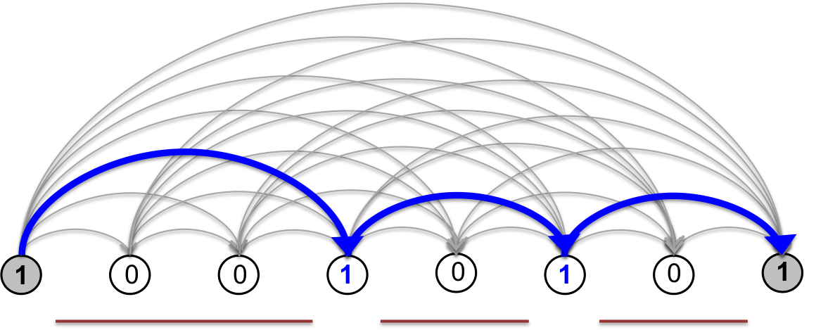
Fig. 5

Nodes can take on states 0 (non-boundary) or 1 (segment boundary). The boundary nodes are the ones visited along a path from the source node to the sink node.

A statistical ensemble

Let’s assume we can associate every possible segment in \(V\) with a score or energy \(E(a,b)\) that tells us how “good” a segment it is. When thinking in terms of energies – as opposed to scores – lower means “better”.

If each segment \([a,b)\) making up a segmentation \(s\) provides an independent energetic contribution, we can define a Hamiltonian for this system as the sum of energetic contributions:

(1)\[H(s) = \displaystyle\sum_{[a,b) \in s} { E(a,b) }\]

Having a Hamiltonian formulation allows us to construct a probabilistic model for the set of all segmentations using the framework of statistical mechanics. We model segmentations in the bit string representation as a thermal system in equilibrium with a heat bath. This statistical ensemble is called the canonical ensemble, where states (segmentations) obey the Boltzmann distribution

(2)\[p(s) = \frac{1}{Z} e^{-\beta H(s)},\]

where the normalization term \(Z\)

(3)\[Z(\beta) = \sum_{s \in S} { e^{-\beta H(s)} } ,\]

is conventionally called the partition function, and \(\beta\) is the inverse temperature with units on the energy scale.

Notable properties of this model:

1. The total energy of a segmentation is the sum of the energies of its segments (1). Its statistical (Boltzmann) weight in the ensemble is given by \(e^{-\beta H(s)}\).
2. The statistical weight of a segmentation is also the product of the Boltzmann weights of its segments, \(e^{-\beta E(a,b)}\).

Essentially, we are treating the occurrences of non-overlapping segments as statistically independent. This assumption allows us to represent the ensemble by assigning arc weights to the segmentation graph. This representation will illuminate efficient methods for obtaining exact solutions for:

• the maximum probability segmentation
• the marginal probability for specific boundaries to occur
• the marginal probability for specific segments to occur
• marginal co-occurrence probabilities of specific nodes in either state (0 or 1)
• independent samples from the ensemble

Depending on the algorithm, the weight we assign to the arc connecting \(a\) and \(b\) is one of

1. segment energy \(E(a,b)\). The total energy of a segmentation \(s\) is then the sum of the arc weights along its path in the segmentation graph.
2. segment statistical weight \(e^{-\beta E(a,b)}\). The statistical weight of a segmentation \(s\) is then the product of the arc weights along its path in the segmentation graph.

The algorithms described below apply to any segment scoring function that satisfies (2). We will explore the results for a segment version of the Potts energy model on Hi-C data.