Algorithms

Optimal segmentation

The most probable segmentation is the one that has the greatest (log) likelihood, or equivalently, is the lowest energy configuration of our system (the ground state). If we place the segment energies on the edges of the segmentation graph, and sum the weights along any given path from source to sink, then this becomes a straightforward case of finding the shortest (longest) path on this directed acyclic graph.

\[s_{\textrm{opt}} = \arg\!\max_{s \in S} \left({ - \displaystyle\sum_{[i,j) \in s} E(i,j)}\right)\]

The optimal segmentation can be found in \(O(N^2)\) time by dynamic programming [Fillipova et al].

\[\begin{split}& H_0 = 0 \\ & H_i = \min_{0 \le k \lt i} \{ H_k + E(k,i-1) \}\end{split}\]

In the graphical models terminology, this algorithm goes by the name max sum. It can be further optimized (linearly bounded) if a maximum segment length is imposed.

Marginal probabilities

Sub-partition functions

Now, if we place the segment statistical weights on the edges of the segmentation graph and take the product of weights along any given path from source to sink, then we can obtain the partition function \(Z(\beta)\) by summing over all paths starting at node \(0\) and ending at node \(N\). Furthermore, we can consider segmentation “subsystems” spanning nodes \(i\) through \(j\) (\(i < j\)) and similarly compute the sub-partition function \(Z_{i,j}\) by summing over paths in that subsystem (see Fig. 6, Fig. 7). The full system partition function \(Z\) is equivalent to \(Z_{0,N}\). We have the following recursion relations:

Forward sub-partition functions:

\[\begin{split}& Z_{0,0} \equiv 1, \\ & Z_{0,t} = \displaystyle\sum_{k=0}^t Z_{0,k} e^{-\beta E(k,t)} \; \forall t \in \{1, \ldots, N \},\end{split}\]

Backward sub-partition functions:

\[\begin{split}& Z_{N,N} \equiv 1, \\ & Z_{N-t,N} = \displaystyle\sum_{k=0}^t Z_{N-k,N} e^{-\beta E(N-t,N-k)} \; \forall t \in \{1, \ldots, N \}.\end{split}\]

This forms the basis of a dynamic programming algorithm that goes by several names: sum-product, forward-backward, belief-propagation, and others.

Marginal boundary probabilities

With these forward and backward statistical weight sums, the marginal probability of each node being a boundary is obtained from

\[p(x_i = 1) = \frac{Z_{0,i} Z_{i,N}}{Z_{0,N}} .\]

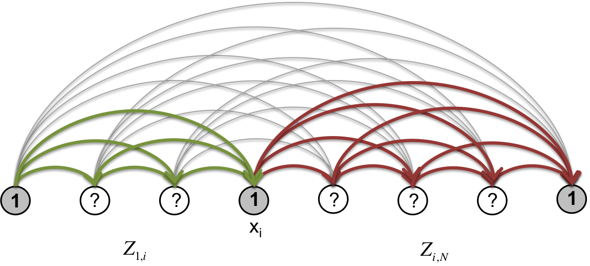
Fig. 6

To get the marginal probability of node \(x_i\) being a boundary, we need to sum over all paths that pass through it. This conditioning reduces the original ensemble to two isolated subsystems, “forward” (green) and “backward” (red).

Hence, although the number of segmentations is exponential in the number of nodes, it is possible to compute the partition function and marginal boundary probabilities in \(O(N^2)\) time.

One can go further and compute the entire set of \(Z_{ij}\) in \(O(N^3)\) and obtain co-occurrence probabilities for all pairs of nodes. The marginal probability of two nodes co-occurring as segment boundaries is given by

\[p(x_i = 1, x_j = 1) = \frac{Z_{0,i} Z_{i,j} Z_{j,N}} {Z_{0,N}}\]

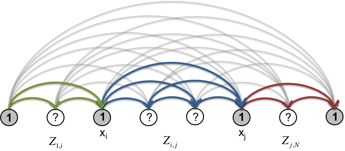
Fig. 7

The subensemble conditioned on two nodes \(x_i\) and \(x_j\) both being boundaries splits the system into three isolated subsystems.

This formula can be generalized to any number of boundaries.

Marginal segment probabilities

We can make use of the forward and backward sub-partition functions to efficiently compute two other quantities of interest.

The marginal probability of the occurrence of a specific segment \([i,j)\) is given by

\[p(x_i = 1, x_j = 1, x_k = 0 \textrm{ for } i \lt k \lt j) = \frac{Z_{0,i} e^{-\beta E(i,j)} Z_{j,N}} {Z_{0,N}}\]

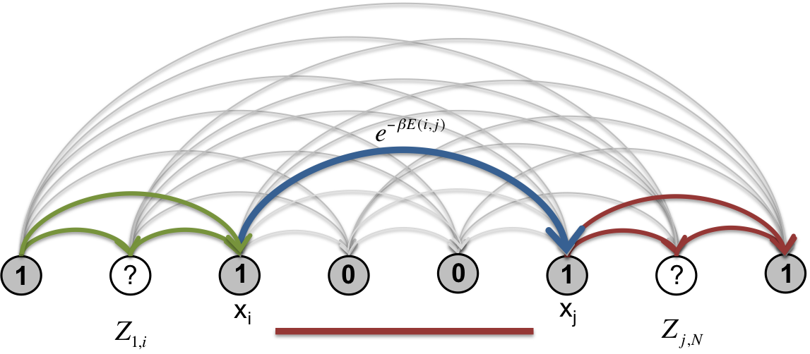
Fig. 8

Conditioning the segmentation ensemble on the occurrence of a specific segment (red line) reduces it to a combination of two isolated subsystems connected by a single arc.

With the forward and backward statistical weights computed as in the previous section, we can further apply dynamic programming to sum up all paths such that \(i\)th and \(j\)th genomic bin co-occur in a common segment. By computing this for all pairs of bins, the resulting marginal segment co-occurrence matrix gives a representation of the ensemble that is easy to compare visually to the original Hi-C matrix. The entire procedure does not exceed \(O(N^2)\).

\[p( x_k = 0 \textrm{ for } i \lt k \le j) = \sum_{p = 0}^i \sum_{q =j+1}^N \frac{ Z_{0,p} e^{-\beta E(p,q)} Z_{q,N}}{Z_{0,N}}\]

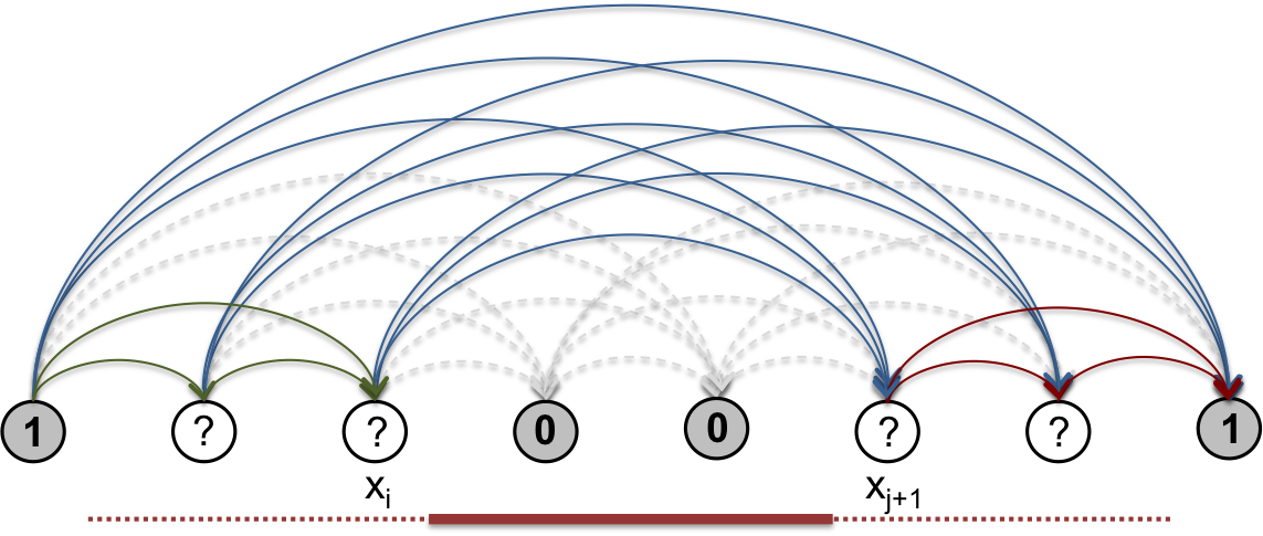
Fig. 9

To condition on bins \([i, i+1)\) and \([j, j+1)\) co-occurring within the same segment, we need to sum over all paths in which nodes \(x_{i+1}, \ldots, x_{j} = 0\).

Sampling

It is possible to obtain independent samples from the ensemble by performing stochastic backtracking walks on the segmentation graph. First, one must pre-compute the forward sub-partition functions. Then to generate samples one proceeds as follows:

• Start at the sink boundary node \(N\). Choose a predecessor boundary node \(k\) from the \(N-1\) available choices by sampling the discrete distribution whose probabilities are given by:

\[p(k \to N) = \frac{Z_{0,k}}{Z_{0,N}}e^{-\beta E(k,N)}\]

• Continue the backward random walk by sampling predecessor nodes \(k'\) until the source node \(0\) is reached.

\[p(k' \to k) = \frac{Z_{0,k'}}{Z_{0,k}}e^{-\beta E(k,k')}\]

Alternatively, one can use the backward subpartition functions and stochastically walk from \(0\) to \(N\).

Hence, samples can be generated without the need for Markov chain-based sampling methods (e.g. Metropolis sampling), which produce correlated samples.